Bomb dive into machine learning – Episode 1

Artificial intelligence today is a topic that is cannibalizing the attention of everyone. From the consumers to the industries, it is revolutionizing many aspects of our lives enabling new abilities, before accessible only to human beings.  ​
​

Despite its media hype, it is often perceived as an advanced argument. Very few people find the motivations to investigate deeper in what is the logic behind the learning mechanisms and quite often definitions like Artificial Intelligence, Machine Learning, and Neural Networks are confused, interchanged or misused in the articles and in the everyday language. 
​
When I first started studying this subject on my spare time, I had the sensation to be in a dark cave, trying to uncover the secrets of machine learning written on a wall pointing at them with a very small torch. It is very easy to find articles and tutorials about specific sub-topics, but it is much more difficult to acquire a general comprehension and vision of this subject.

In the next sections of this blog, we will clarify some main concepts and use them to generate a system that can predict the height of every sportsman! 
 
Artificial Intelligence vs Machine Learning vs Neural Networks 
​(a.k.a. Deep Learning) 
Artificial intelligence is a generic definition that refers to all the techniques and algorithms capable to perform intelligent tasks (i.e. image recognition). It includes both all the classical approaches in which the logic of the program is explicitly defined (coded) and the ones in which the logic is learnt from the observation of a very big set of data. 

Machine learning describes a set of techniques and algorithms capable of learning from a set of data provided in input. The machine learning algorithms are a sub-class of the artificial intelligence “world”. 

Neural Networks, often referred as Deep Learning, emulate a simplified structure of our brain connecting in cascade several layers of digital neurons (called tensors). During a training phase, the tensors are able to learn from a big set of data, so the Neural Networks are part of the Machine Learning category. 

In this article, we will focus on the Machine Learning techniques.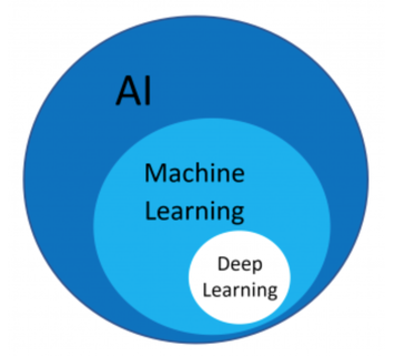 

What is the main subject? 
Something that is not immediate when we talk about Machine Learning is also the main subject of the discussion. Are we discussing about some sort of development framework for programmers, a subfield of statistical sciences or a pure mathematical tool?  

​The true stands in the middle of all this statements. Machine Learning as subject is like a big mountain that can be admired from different perspectives. To conquer its peak, we need to get first comfortable with its different sides, approaching it with both a statistical/mathematical and a developer vision. ​

Supervised learning & Linear Regression 
We previously mentioned that every machine learning algorithm need a big set data in input in order to start the learning process. Depending on the data provided in input, these algorithms could be further divided in other 2 sub-categories: 

• Supervised Learning: All data is labeled and the algorithms learn to predict the output from the input data 
• Unsupervised Learning: All data is unlabeled and the algorithms learn to inherent structure from the input data

Everything we need to know for now is that in the next sections we will see in detail a particular method that is part of the Supervised Learning category: the Linear Regression. 
 
A practical example 
So far, we clarified a lot of main concepts, now it is time to get practical!  

Let’s imagine a sportswear company that is going to launch a new series of technical clothing that covers most of sports represented in the Olympic games. They want to overcome the competitors creating custom sizes and providing the best fit in the market for every sport. 

​To do so, they need to generate a model to see how the body of the athletes evolves through different sports, ages and weights.  

To better clarify this concept, we could compare a judo athlete and a basketball player. If they both weight 90 Kg, the judo athlete will likely be more muscular and shorter than the basketball player (this sport notoriously requires a higher stature and a medium fitted body to do not waste too much energy during the match).  
​
In this example, we will focus on predicting the height of the athletes, the same principles could be used also to predict any other important metric for the size like the shoulder distance etc. 
 
Dataset wanted 
The first step is the most important one: it will be the pillar of every following action and an error in this phase will likely invalid any further effort to improve the prediction accuracy. We need to find a dataset containing at least the following information about the athletes: 

• Age 

• Weight 
• Sport 
• Height 

A good place to start is … yes, it is always him, Mr. Google but, in this case, we are not going to use its classic version. At the day of this article, google is providing a specific search engine (in beta version) dedicated to the datasets, it is available at the link https://toolbox.google.com/datasetsearch

Searching the terms “Olympic athletes”, the third result returns a public dataset published on Kaggle (https://www.kaggle.com/rio2016/olympic-games) which contains a list of the athletes that attended the last Olympic games in Brazil. A quick look at the data preview reveals that it contains everything we need and even more, so we found our dataset! 

Linear Regression  
After choosing the dataset we have to make another important decision: which model to use to tackle the problem.  
​
Analyzing the requirements, our system needs to provide a continuous prediction of the height, conditioned by 3 variables (age, weight and sport). This kind of challenges can be approached with good results using a model called Linear Regression. 

To keep the things easy, let’s consider only 2 columns of our dataset: the height and the weight of the athletes. If we plot in a graph these fields for every athlete in our dataset we will obtain the following: 

From this graph, it is immediately noticeable that a sort of linear relation exists between weight and height (logically it make sense).  The linear regression model is able to find the best-fitting line, that is the line that minimizes the distance between the points and their projection on the line.  

Graphically, it looks like the following: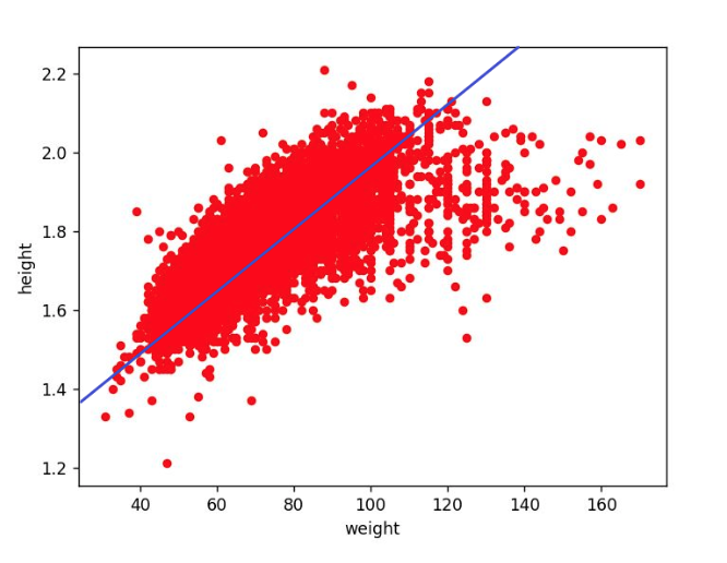

This line is represented by the academic formula:  
Y = mX + q 
Or, in our example: 
Height = m * Weight + q 

The goal of our model is to find the right combination of the parameters { m, q } that can produce the best-fitting line applied to all the points in our dataset. These parameters will be “learned” during the training phase of our model. 
 
How does it learn? 
The learning magic happens during the training phase: in this part of the process the Linear Regression model is provided with all the data (or, to be more precise, with most of the data, as we will explain in the following sections) in the dataset. Automatically the model tunes its internal parameters { m , q }, getting progressively more accurate until it does not achieve the best-fitting line. 
 
How is it able to tune its internal parameters by itself?    
Considering our example, before the training we would have our model represented by the formula: 

Height = m * Weight + q 

with the internal parameters { m , q } initialized with the values { 0 , 0 }. 
Then, we start the training, providing in input to the model the height and weight of every athlete in the dataset. 

For every athlete, the model: 

1. Creates its prediction for the height, that at the beginning will be: HeightPred = 0 * Weight + 0 = 0. 
2. Calculates the error of the prediction, comparing it with the Height provided in input. At the beginning, it will be: Error = | HeightPred – Height | = | 0 – Height | = Height. 

​After finding the error for every prediction for every athlete, we can calculate the average error relative to the parameters { 0 , 0 }. 

Let’ s now imagine to assign the parameters { m ,q } with every possible value they can assume, calculate the average error over all the predictions, and plot it in a 3 dimensional graph. The result would look like the following:  ​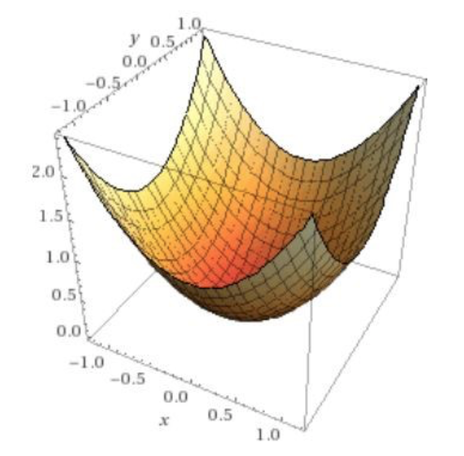

We can notice from the graph that there is a point in which the average error is minimum. This is exactly the point that we want to reach, or more correctly, the model needs to find the value of the parameters { m, q } associated with this point of minimum. 
​
Trying all the possible values is clearly not a feasible option, luckily there are different strategies that we can adopt to find this point in a more efficient way. 
 
Gradient descent 
Getting back to our example, we have seen that when the training is first started { m , q } are initialized to { 0, 0 } and they produce a certain average error (very high). 

At this point the model should update its internal parameters to decrease the average error in the next round of predictions.  

A very common strategy is called Gradient descent, the main idea behind it is that the point of minimum can be found following progressively the direction of the derivative of the error, making the parameters falling in the point of minimum like a ball rolls down a valley. 
​
Applying it to our example, after calculating the average error with the parameters { 0, 0 } the steps are: 

1. Calculate the partial derivative of the average error at the point { 0, 0 }. 
2. The derivative returns the slope of the error on that point. To move toward the point of minimum we can than follow the slope finding a new point in that direction. 
3. Project the new point to the m and q axis, in this way it is possible to find the values { delta_m, delta_q } to apply to the parameters { m, q }. 
4. Update the internal parameters { m , q } with the previously calculated values: { m+delta_m, q+delta_q }. 

​
For a more detailed explanation, with also all the real math involved, the following article will not let you down for sure:  https://towardsdatascience.com/machine-learning-101-an-intuitive-introduction-to-gradient-descent-366b77b52645.   ​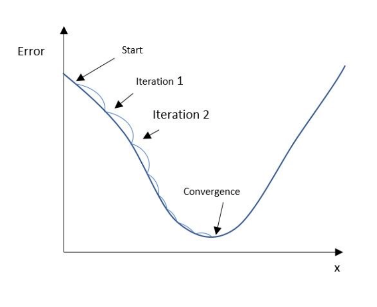

 
General outcomes 
In the previous section we modeled the Linear Regression with only 1 argument in input ( the weight ). The same concepts are still valid when we add other arguments, the general formula of the model in this case becomes: 

Inputs= { X1, X2, … Xn } 
Parameters = { W1, W2, … Wn , b } 
Y = W1 * X1 + W2 * X2 + … + Wn*Xn + b 

Many concepts that we have seen in the previous sections can be globally applied to every machine learning project. The steps can be generalized as follows: 

1. Clarify all the requirements 
2. Find a dataset containing all the information needed (or build it using different sources) 
3. Choose a model that can properly fit the problem tackled 
4. Define how the error on the predictions is calculated (finding a cost function) 
5. Define the strategy used to find the minimum of the error 

Conclusion
Well done, you just successfully examined an enormous number of concepts, from the real meaning of the machine learning definition to the mathematical world that lives underneath. 

In this journey, we traveled on a high-speed train, preferring the final destination (a general understanding of all the main concepts involved) over the single stations in the middle.  

As in small, pretty towns, these stations can have a lot to offer and it might be worth visiting if you can spend a little extra time on your trip: 

• AI vs ML: www.forbes.com/sites/bernardmarr/2016/12/06/what-is-the-difference-between-artificial-intelligence-and-machine-learning/#5754193a2742
• Supervised, Unsupervised and Semi-supervised Learning: https://blogs.nvidia.com/blog/2018/08/02/supervised-unsupervised-learning/ 
• Dataset preparation: https://developers.google.com/machine-learning/data-prep/ 

• Linear Regression: https://towardsdatascience.com/linear-regression-detailed-view-ea73175f6e86 
• Gradient descent: https://towardsdatascience.com/gradient-descent-in-a-nutshell-eaf8c18212f0 
  
  

In the next episode 
In the second episode, we will see how everything we learned so far can be translated in a python code. We will then implement together the sportsman height predictor we idealized in our examples.  Stay tuned and see you soon with the second episode! 
 

Davide Poveromo 
Software Engineer

Davide works as a software engineer for HCL Technologies.  
​
He loves web in all its dialects. Developing web services and applications is Davide’s huge passion. Solving real world problems using the potential of the networks is one of the most satisfying sensations for him. Recently, Davide is working on machine learning models and blockchain technology.