Quantitative evaluation of the scalability of the Workload Automation system with a web UI front-end

This article shows an approach for the quantitative evaluation of the scalability of a system with a web UI front-end, which has been applied to the HCL Workload Automation product during the performance verification test phase.

The article is divided into the following sections:

• Introduction
• Quantifying Scalability
• Generating variable load
• Example application
• Conclusion
• Appendix: Using Excel’s Solver add-in to fit the USL to performance data

Introduction 
A generic approach to evaluate the scalability of a system could consist of the following tasks:

• collection of available performance and scalability requirements
• definition of the system under test, in terms of hardware, software, and application configuration, according to the requirements
• definition of the test workload to run against the system under test, in terms of required test data, selection of application features to include in the tests, request rates or number of concurrent requests to send to the system
• execution of load tests at different load levels, or with different system configurations
• test results analysis

This approach can be used to perform a quantitative assessment of the scalability of a system by building a simple analytical model using Little's law and the “Universal Scalability Law” (USL).
 
There are many available load generation tools that can be used to execute load tests, with different load levels, against a system with a web UI. In the example shown later, the tool used is HCL OneTest Performance.
 
While tasks from 1) to 3) depend on the specific system under test, tasks 4) and 5) can be described in general terms. The proposed approach for tasks 4) and 5) is explained using the Dynamic Workload Console (DWC), a web-based user interface for HCL Workload Automation (WA), as an example of a system with a web UI.

Quantifying Scalability 
When running load tests against a system, the three performance metrics that need to be collected and analyzed are:

• Throughput (X): the rate at which the system is processing requests
• Response time (R): the time required by the system to process a request
• Load or Concurrency (N): the number of requests that the system is processing concurrently

 
For each test at a given load level, the load must be applied to the system long enough for the it to reach a stationary state, and to collect a statistically significant number of samples in this steady state.
For a system in steady state, the long-term average values of the three metrics obey to Little's law:

​Little’s law can be used to calculate the value of one of the three metrics when only two of the other values are available.
 
In many cases, the measured or calculated values of X and N at the different load levels (X1, N1, X2, N2, … Xn, Nn), will follow the “Universal Scalability Law” (USL):

​Fitting the USL to the measured values of X and N allows for the calculation of the three coefficients:

• γ: the coefficient of performance, which represents ideal parallelism or “efficiency”
• α: the coefficient of contention, which represents serialization or queueing
• β: the coefficient of crosstalk, which represents coherency/consistency/synchronization

 
The values of α, β, γ quantify the scalability of the system under test.
 
The theoretical maximum concurrency level (Nmax) can be determined with the formula:

From this value, the theoretical maximum throughput (Xmax) can be calculated using the fitted USL:

Once a set of at least 6 (the more, the better) couples of values (X, N) has been determined, one for each test run at a given load level, it is possible to fit the USL to them; for instance using Excel’s Solver add-in as explained in Appendix: Using Excel’s Solver add-in to fit the USL to performance data.
 
The Universal Scalability Law is a simple, black-box approach that models the system as a whole. It is based on simple relationships that hold true in most conditions. As such, it has limitations: for example, the USL carries no notion of heterogeneous workloads, like those occurring in a production environment, which involve different user types executing different business functions. Nevertheless, even in some such cases, the USL has been applied successfully, allowing the definition of a simple, quantitative model of a system’s scalability.

Generating variable load 
HCL OneTest Performance is a workload generator tool, based on Rational Performance Tester, for automating load and scalability testing of web, ERP, and server-based software applications. It captures the network traffic that is rendered when the application under test interacts with a server. This network traffic is then emulated on multiple virtual users while playing back the test. During playback, server response times, throughput, and other measurements are collected, and related reports are generated.
 
Load tests for a web application are built by recording a set of actions performed on the web UI itself, using a browser configured to have OneTest Performance capture all the data flowing between the browser and the application.
 
A recording creates multiple HTTP requests and responses, which will be grouped by OneTest Performance into “HTTP pages”.
Each HTTP page contains a list of the requests recorded for that page, named after their web addresses.
A HTTP request contains the corresponding response data.
Collectively, requests and responses listed inside a HTTP page are responsible for everything that was returned by the web server for that page.
 
By defining user groups, related tests can be grouped, and run (i.e., played back) in parallel: tests belonging to different user groups run in parallel.
 
By adding a test to a Schedule, it is possible to emulate the action of an individual user.
A schedule can be as simple as one virtual user or one iteration running one test, or as complicated as hundreds of virtual users or iteration rates in different groups, each running different tests at different times.
 
A schedule can be used to control tests, and the load level they generate against the system, in the following ways:

• Group tests under user groups, to emulate the actions of different types of users or rates
• Set the order in which tests will run: sequentially, randomly, or in a weighted order
• Set the number of times that each test runs
• Run tests at a certain rate
• Run tests for a certain time, and increase or decrease virtual users or rate during the run

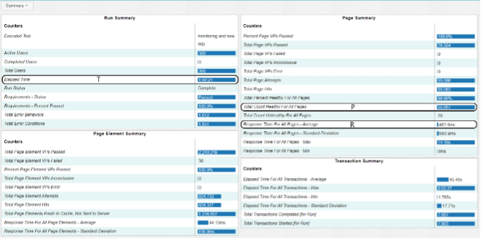
Example application 
The Dynamic Workload Console (DWC) is a web-based user interface for HCL Workload Automation (WA). OneTest Performance can be used to record and play back tests for DWC.
After the execution of a test schedule, at a specified load level, is completed, OneTest Performance will generate a report with a summary page like the following:

Numbers shown above are just an example and are not meant to document a specific DWC performance level)
 
The performance metrics X and N can be calculated from the summary report using the values of:

• “Elapsed Time” (T): this is the test run duration, which is displayed in hours, minutes, and seconds
• “Total Count Healthy For All Pages” (P): this is the number of primary requests that hit the system, received a complete response, and are included in pages that did not report errors for any of their elements (“healthy”)
• “Response Time For All Pages - Average” (R): this is the average of the response times for all pages. A page response time is the sum of response times for all page elements. Response time counters omit page response times for pages that contain requests with status codes in the range of 4XX (client errors) to 5XX (server errors). The only exception is when the failure (for example, a 404) is recorded and returned, and the request is not the primary request for the page. Page response times that contain requests that time out are always discarded

 
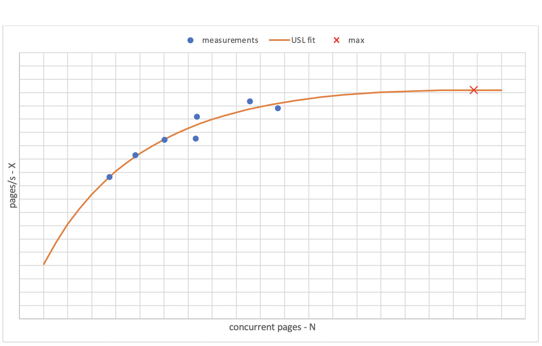
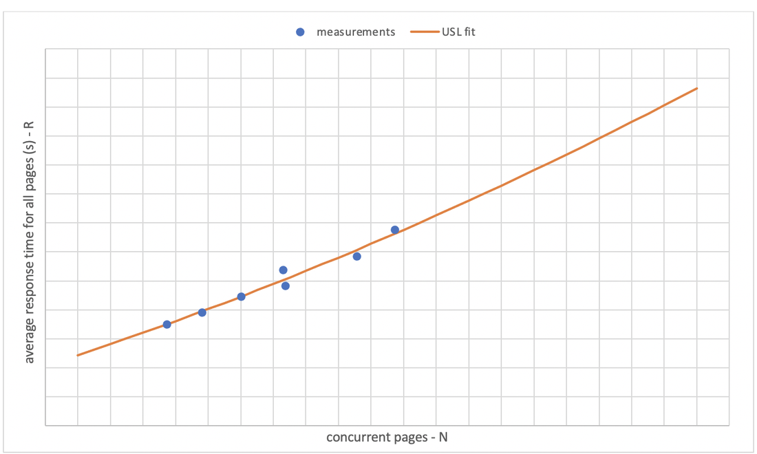
Given the value of T, P, and R, X and N can be calculated using:

Running the same test multiple times, each time configuring the schedule with a different number of users or with different rates, allows to measure different values for (X, N).
As an example, the following chart shows a set of 7 measurements (X, N), corresponding to 7 different runs of the same test schedule, and the corresponding USL fit:

Once the values of α, β, γ are available, it is also possible to model the relationship between average response time (R) and concurrency (N), by application of Little’s law and USL:

The following chart shows an example for the same data as above:

Conclusion 
This article shows how to build a simple quantitative scalability model of a system with a web UI front-end using a workload generator tool. As an example, HCL OneTest Performance can be employed to collect performance data for a system like DWC; these data can then be used to build such a model.
 
Despite its simplicity and limitations, the USL provides a quantitative framework for:

• Validating test measurements – measurements that don’t fit the model need to be questioned
• Comparing test results with expectations
• Comparing test results collected under different HW or SW configurations
• Predicting how a system will perform under loads beyond those measured
• Explaining why a system isn’t scaling well

 
 Appendix: Using Excel’s Solver add-in to fit the USL to performance data
 
Using the Universal Scalability Law (USL) to quantify the scalability of a system requires the estimation of the three coefficients α, β, γ for the equation:

This is achieved by fitting the curve X(N) to the measured performance data (N, X) using non-linear least squares regression analysis.
 
In addition to general purpose libraries that implement some of the algorithms commonly used to perform non-linear least squares regression analysis (e.g., the least squares package in Apache Commons Math or the optim package for GNU Octave), there are also freely available programs that can be used to carry out the computation; for example:

• an R package to analyze system performance data with the Universal Scalability Law
• implementations in Java, Go, and Rust

 
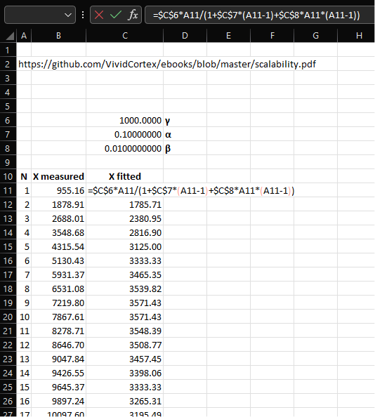
However, if the number of measurements to fit is not large, it also possible to estimate α, β, γ using Microsoft Excel’s Solver add-in, without writing any code.
 
The steps to calculate the values of α, β, γ that fit the measurements are:

• insert the measured values of N, X into two columns of a spreadsheet
• set initial values for α, β, γ in three cells
  • for γ, choose a value close to the measured value of X(1)
  • for α, choose a value between 0 and 1, closer to 0 rather than 1 (e.g., 0.1 or 0.05)
  • for β, choose a value greater than zero and lower than α (e.g., 0.01 or 0.005)
• fill in a column with the calculated values of X based on the initial values for α, β, γ and the measured values of N, using equation 1)
  
• insert a formula in a cell to calculate the sum of squares of the differences between the measured value of X and the calculated value of X (the sum of squared residuals):

• open the Solver dialog, choose the cell holding the residual sum of squares as the “objective” to minimize, and the three cells with the initial value for α, β, γ as the “variable cells”
  • check the “Make Unconstrained Variables Non-Negative” checkbox
  • the “Generalized Reduced Gradient (GRG) Nonlinear” method should work most of times
  • if the solution proposed by the Solver is obviously wrong, it might be necessary to set constraints for α≤1 and β≤1 and re-run the Solver with the original values of α, β, γ
  • other Solver options that seem to improve convergence:
    • “All Methods” tab: Use Automatic Scaling
    • “GRG Nonlinear” tab: Convergence – set its value to the precision you want to reach
    • “GRG Nonlinear” tab: Central Derivatives
    • “GRG Nonlinear” tab: Use Multistart
• keep running the Solver as long as the solution is converging; stop it as soon as the solution diverges
• optionally choose to create a Solver report sheet

 
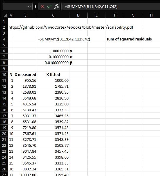
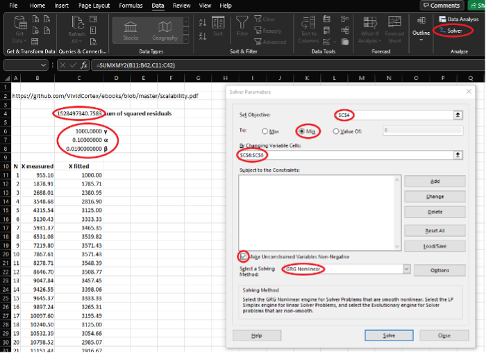
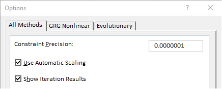
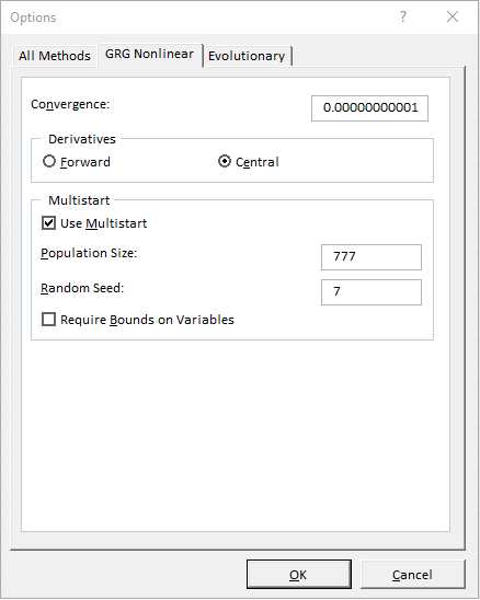
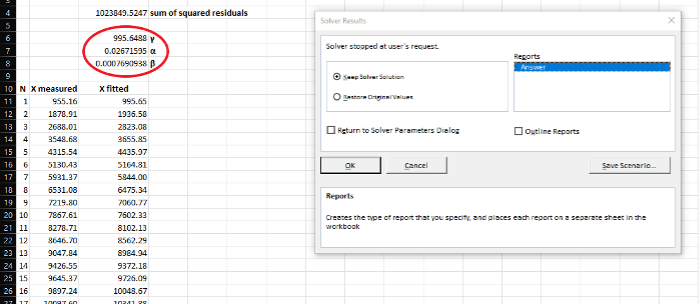
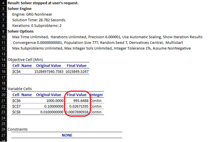
A similar approach can be used with LibreOffice Calc’s Solver.
 
To prove the practical applicability of the approach, the following section shows how to use Excel’s Solver to calculate the values of α, β, γ and compares them to the values generated by other methods for the same sets of measurements.
 
Examples with known results (α, β, γ) The book Practical Scalability Analysis with the Universal Scalability Law by Baron Schwartz contains an example application of the USL to the results of running the sysbench benchmark on a Cisco UCS C250 rack server, in chapter “Measuring Scalability” at page 15.

The following screenshots show how to use Excel and its Solver add-in to calculate the best-fit values of the three coefficients in the USL formula for the performance data documented in that chapter.

After having implemented steps 1, 2, and 3, the spreadsheet should look like this:

​The next screenshot shows the formula for step 4:

​The main elements for steps 5, 5a, and 5b are highlighted in the following screenshot:

Additional Solver options mentioned in step 5d are shown by the next two screenshots:

​The next screenshot shows the final state of the spreadsheet, after having stopped the Solver at the first iteration whose result diverged:

​Excel’s Solver last dialog offers the option to generate an “answer report” (step 7), which consists of a sheet with information about the Solver set-up and execution:

The results yielded by the Solver are very close to the documented results, calculated using R language’s nls function, which are:

• γ = 995.6486
• α = 0.02671591
• β = 0.0007690945

 
Two other examples can be found in the documentation of the usl R package, in sections “4.1 Case Study: Hardware Scalability” and “4.2 Case Study: Software Scalability”. These examples are provided by the package itself as demo datasets.
 
Following the same steps described above, for the first example (Hardware Scalability), the results are:

Note that for this example to reach convergence it might be necessary to add constraints for α≤1 and β≤1.
 
For the second example (Software Scalability), the results are:

​These three examples show that it is possible to use Excel’s Solver add-in to quicky find values of α, β, γ that fit the USL to a set of performance measurements, with a precision similar to that of available implementations of non-linear least squares regression analysis algorithms.

---

Authors Bio

Paolo Cavazza - Lead Software Engineer
Paolo joined HCL Software in December 2020 to work with the Workload Automation Test Team as a Performance Tester.